Bayesian Modelling

This blog post talks about methodology of building Bayesian models.

We discussed the below model in the previous post. In this model -

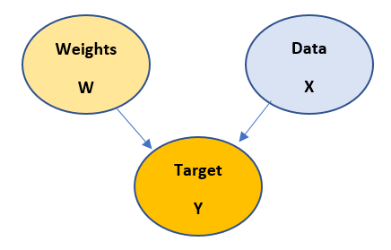
1. when there is an arrow pointing from one node to another, that implies start nodes causes end node. For example, in above case Target node depends on Weights node as well as Data node.
2. Start node is known as Parent and the end node is known as Child
3. Most importantly, cycles are avoided while building a Bayesian model.
4. These structures are generated from the given data and experience
5. Mathematical representation of the Bayesian model is done using Chain rule. For example, in the above diagram the chain rule is applied as follows:
P(y,w,x) = P(y/w,x)P(w)P(x)
Generalized chain rule looks


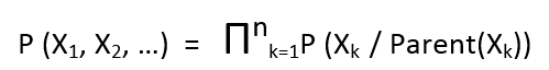
6. The Bayesian models are build based upon the subject matter expertise and experience of the developer.

Example

Given are three variables - sprinkle, rain , wet grass, where sprinkle and rain are predictors and wet grass is a predicate variable, how would we design a Bayesian model for it.

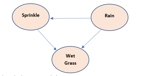
• Sprinkle is used to wet grass, therefore Sprinkle causes wet grass so Sprinkle node is parent to wet grass node
• Rain also wet the grass, therefore Sprinkle causes wet grass so Rain node is parent to wet grass node
• if there is rain, there is no need to sprinkle, therefore there Is a negative relation between Sprinkle and rain node. So, rain node is parent to Sprinkle node

Chain rule implementation is :

P(S,R,W) = P(W/S,R)*P(S/R)*P(R)

Introduction to Latent Variable

According to Wiki, in statistics, latent variables (from Latin: present participle of lateo (“lie hidden”), as opposed to observable variables), are variables that are not directly observed but are rather inferred (through a mathematical model) from other variables that are observed (directly measured).

Latent variables are hidden variables i.e. they are not observed. Latent variables are rather inferred and are been thought as the cause of the observed variables. In Bayesian models they are used when we end up in cycle generation in our model. They help us in simplifying the mathematical solution of our problem, but this is not always correct.

Suppose we have a problem , hunger, eat and work, and if we create a Bayesian model, it would be something like -

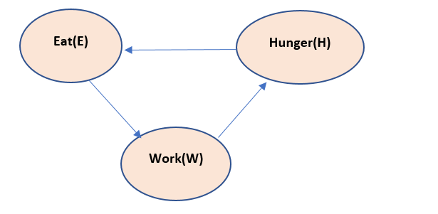
The above model reads like, if we work, we feel hunger. If we feel hunger – we eat. If we eat, we have energy to work.

Now this above model has a cycle in it and thus if chain rule is applied to it, the chain will become infinitely long. So, the above Bayesian model is not correct. Thus, we need to introduce the Latent variable here, let us call it as T.

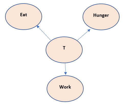
Now the above mode states that, T is responsible for eat, hunger and work to happen. This variable T is not observed but can be inferred as the cause of happening of work, eat and hunger. This assumption seems to be correct also, as in a biological body – something resides in it that pushes it to eat and work, even though we cannot observe it physically.

Let us write the chain rule equation for the above model:

P(W,E,H,T) = P(W/T)*P(E/T)*P(H/T)*P(T)

Let us see another example. Suppose we have following variables: GPA, IQ, School. The model reads like if a person has good IQ, he/she will get good School and GPA, if he/she got good School, he/she will have good IQ and may get good GPA. If he/she gets good GPA, he/she may have good IQ, and he/she may be from good School. The model looks like:

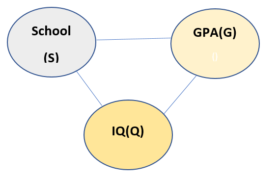
Now from above description of the model, all the nodes are connected to every other node. Thus chain rule cannot be applied to this model. So we need a Latent variable to be introduced here. Let us call the new Latent variable as I. The new model looks like:

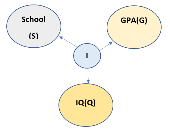
Now we read the above model as Latent variable I is responsible for all the other three variables. Now the chain rule can easily be applied. And it looks like:

P(S,G,Q,I) = P(S/I)*P(G/I)*P(Q/I)*P(I)

So, we can see that latent variables help in reducing the complexity of the problem.

The next post will highlight Bayesian inferencing using the latent variables wherever required.

How many clusters will be formed?

Let us take a sample data set visual :

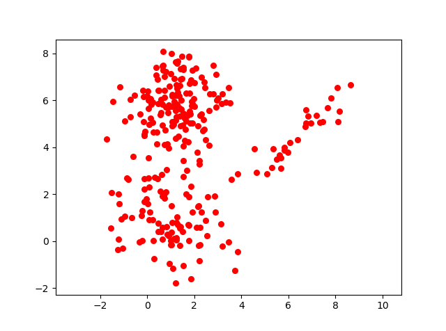
Upon close observation, one can see that there are 3 clusters in it. So, lets define these 3 clusters probabilistically.

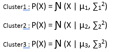
Now, let us try to write an equation which can define the probability of a point in the data to be a part of every cluster. But before that, we need a mechanism or a probability function that can define which cluster a point can be from and with what probability. Let us say that a point can be a part of any cluster with equal probability of 1/3. Then the probabilistic distribution of a point would look like:

But in the above case, it is an assumption that every point can belong to any cluster with equal probability. But is that correct? No! So, let’s use a Latent Variable which knows the distribution of every point belonging to every cluster. The Bayesian model looks like:

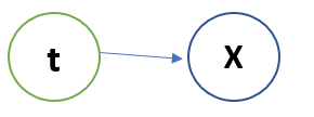
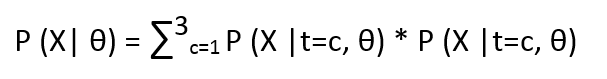
The above model states that Latent Variable t knows, to which cluster the point x belongs and with what probability. So, if we re-write the above equation, it looks like -

Now let us call all our parameters as

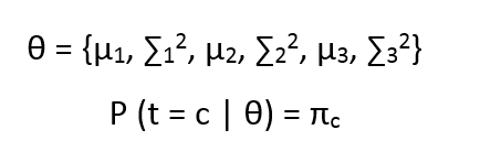
the above equation states that the probability by which the Latent variable takes value c, given all the parameters is πc

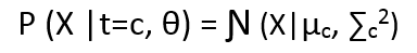
The above equation states that probability of a point sampled from cluster c, given that it has come from cluster c is Ɲ (X|µc, ∑c2).

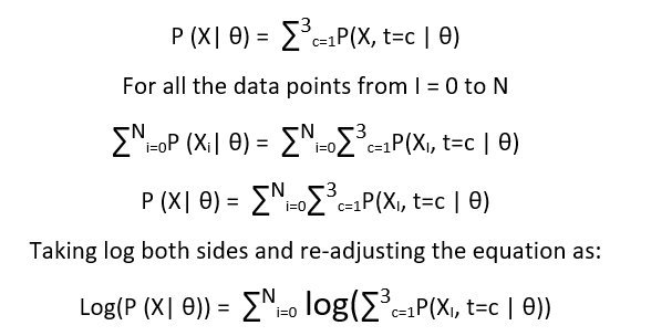
Now we know that P(X, t=c | θ) = P(X| t=c, θ) * P(t=c | θ) from our Bayesian model. We can marginalize t to compute

The above equation is exactly same as our original one.

Fact Checks

Where LHS is the posterior distribution of t w.r.t X and θ. Z is the normalization constant and can be calculated as :

The Chicken-Egg Problem in Probabilistic Clustering

Now we are clear that in the Bayesian model we made between t and x, when we say the latent variable knows the cluster number of every point, we say it probabilistically. This means the formulae applied is the posterior distribution, as we discussed in Fact check section. Now the problem is, to compute θ, we should know t and to compute t, we should know θ. We will see this in the following equations:

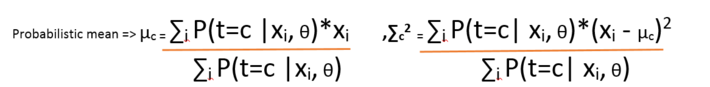
And the posterior t is computed using

The above expression clearly shows that means and standard deviations can be computed if we know the source t and vice-versa.

The next post will show how to solve the above problem using Expectation Maximization algorithm.

Expectation – Maximization Algorithm

From our previous blog discussion, we know that marginalized posterior distribution looks like -

Now we need to maximize the above expression w.r.t θ. The problem here is that maximization of the above expression is not simple, as function usually has many local maxima. We can use gradient – decent here but it will make the process long. To solve this, we use a different approach - we will try and construct a lower bound of the above expression using Jensen’s inequality. And once we build our lower bound, we will try and maximize it.

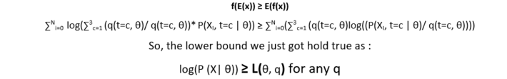
The lower bound is also called variational lower bound and we are applying Jensen’s inequality to compute the lower bound. Consider the log as our function f and let us introduce a new function q(t=c, θ), and multiply it in denominator and numerator. So the new equation looks like:

Now consider the ratio (P(XI, t=c | θ)/ q(t=c, θ)) as random variable and q(t=c, θ) as the probabilistic coefficient as ∑3c=1 q(t=c, θ) = 1.

Now from Jensen’s inequality, we know that:

Graphically,

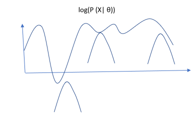
All the above small curves are the derived from lower bound L(θ, q).

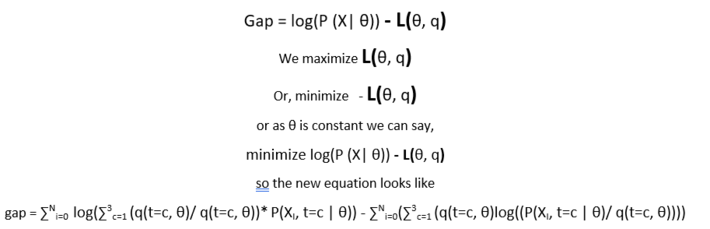
Expectation Step

It is clear that the lower bound will always be beneath the actual function, and we need to maximize the lower bound to be as much closer to actual function as possible. In expectation step we fix our θ and try to maximize the lower bound. We do it by reducing the gap between actual function and the lower bound. The equation is as follows :

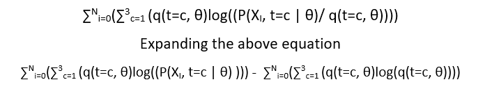
putting in some linear algebra, the equation ends up in the expression of KL divergence between q and posterior t

The solution of expectation step is :

q(t=c) = P(t=c | Xi ., θ)

Maximization step

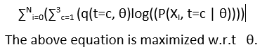
Once we get the gap reduced between the variational lower function L(θ, q) and log(P(X |θ)), we maximize our lower bound function w.r.t θ.

The second component of above equation is constant w.r.t θ. Therefore, we drop it, the new equation remains is:

In the next post we will continue our discussion and introduce Gaussian mixture model. We will see how to implement Expectation – Maximization algorithm to perform clustering.

This point of view article originally published on datasciencecentral.com. Data Science Central is the industry's online resource for data practitioners. From Statistics to Analytics to Machine Learning to AI, Data Science Central provides a community experience that includes a rich editorial platform, social interaction, forum-based support, plus the latest information on technology, tools, trends, and careers.

Click here for the article