This post is about how Expectation-maximization algorithm. It is in continuation of the previous blog that showed how probabilistic clustering ended up into chicken-egg problem. That is, if we have distribution of latent variable, we can compute the parameters of the clusters and vice-versa. To understand how the entire approach works we need to learn few mathematical tools, namely Jensen’s inequality and KL divergence.

Jensen’s Inequality

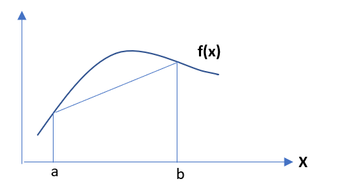
Jensen’s inequality states that, for a convex function f(x) , if we select points as x = a and x = b, also we take α,β such that α + β = 1 ,then

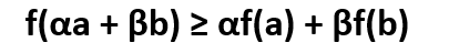
If we consider x as a random variable and it takes the values a, b with probability α, β (as we know α + β = 1), then the expression αa + βb is the expectation of x –> E(x), and the expression αf(a) + βf(b) -- > is E(f(x)). Thus, the expression of Jensen’s inequality can be re-written as:

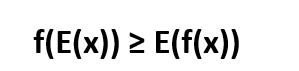
This above expression will be used in further analysis.

Kullback–Leibler divergence

This is the method of computation of divergence between two probability distribution functions. The mathematical expression is as follows:

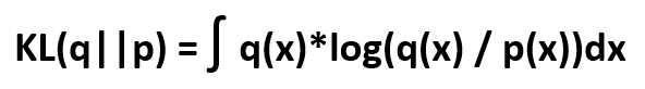
Where q(x) and p(x) are pdf. functions on a random variable x. KL(q||p) is always ≥ 0.

Expectation – Maximization Algorithm

From our previous blog discussion, we know that marginalized posterior distribution looks like -

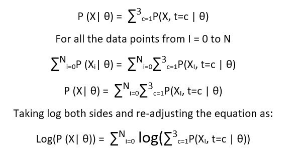
Now we need to maximize the above expression w.r.t θ. The problem here is that maximization of the above expression is not simple, as function usually has many local maxima. We can use gradient – decent here but it will make the process long. To solve this, we use a different approach - we will try and construct a lower bound of the above expression using Jensen’s inequality. And once we build our lower bound, we will try and maximize it.

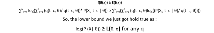
The lower bound is also called variational lower bound and we are applying Jensen’s inequality to compute the lower bound. Consider the log as our function f and let us introduce a new function q(t=c, θ), and multiply it in denominator and numerator. So the new equation looks like:

Now consider the ratio (P(XI, t=c | θ)/ q(t=c, θ)) as random variable and q(t=c, θ) as the probabilistic coefficient as ∑3c=1 q(t=c, θ) = 1.

Now from Jensen’s inequality, we know that:

Graphically,

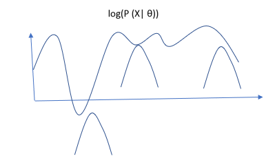
All the above small curves are the derived from lower bound L(θ, q).

Expectation Step

It is clear that the lower bound will always be beneath the actual function, and we need to maximize the lower bound to be as much closer to actual function as possible. In expectation step we fix our θ and try to maximize the lower bound. We do it by reducing the gap between actual function and the lower bound. The equation is as follows :

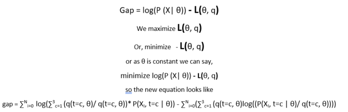
putting in some linear algebra, the equation ends up in the expression of KL divergence between q and posterior t

The solution of expectation step is :

q(t=c) = P(t=c | Xi ., θ)

Maximization step

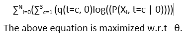
Once we get the gap reduced between the variational lower function L(θ, q) and log(P(X |θ)), we maximize our lower bound function w.r.t θ.

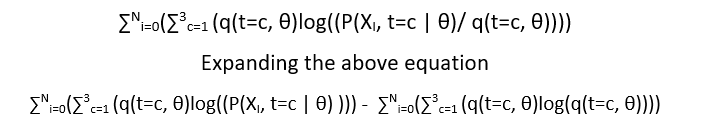
The second component of above equation is constant w.r.t θ. Therefore, we drop it, the new equation remains is:

In the next post we will continue our discussion and introduce Gaussian mixture model. We will see how to implement Expectation – Maximization algorithm to perform clustering.

This point of view article originally published on datasciencecentral.com. Data Science Central is the industry's online resource for data practitioners. From Statistics to Analytics to Machine Learning to AI, Data Science Central provides a community experience that includes a rich editorial platform, social interaction, forum-based support, plus the latest information on technology, tools, trends, and careers.

Click here for the article