Continuing the discussion on probabilistically clustering of data, and after understanding the modelling theory of Expectation – Maximization algorithm, its time to implement it.

Referring to the same problem, where we had assumed 3 clusters.

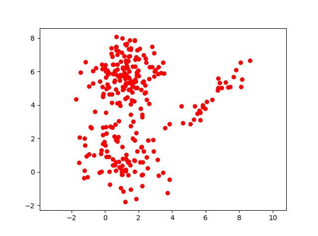
For each of the 3 clusters, the Gaussain distribution can be defined as follows :

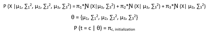
We also discussed that data came from a Latent variable t that knows which data point belongs to which data point with what probability.

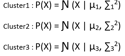
The Bayesian model looks like :

Now the probability of the observed data given the parameters looks like :

The point to note here is that the equation below is already in its lower bound form, so no need to apply Jensen’s inequality.

E-Step

As we know, the E-step solutions is :

q(t=c) = P(t=c | Xi ., θ)

Since there are 3 clusters in our case we will need to compute the posterior distribution for our latent carriable t for all the 3 clusters.

We will apply the above equation for all the observed data points, for every cluster with respect to every point. For example, we have 100 observed data points and 3 clusters, then the matrix of the posterior on the latent variable t is of dimension – 100 x 3.

M-Step

In the M step, we maximize our lower bound variational inference w.r.t θ and use above computed posterior distribution on our latent variable t as constants.

The equation we need to maximize w.r.t θ and π1 ,π2 , π3 , is:

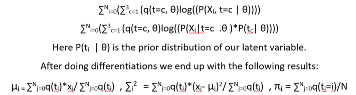
The priors are computed with constraint that every prior >= 0 and sum of all
prior = 1
The E step and M step are iterated a multiple times, one after the other, in a fashion that results of E step are used in M step and results of M step are used in E step. We end the iteration when the loss function stops reducing.
The loss function is the same function which we are differentiating in the M step.
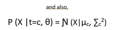
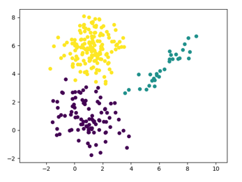
The result of applying the EM algorithm on the given data set is as below:

This point of view article originally published on datasciencecentral.com. Data Science Central is the industry's online resource for data practitioners. From Statistics to Analytics to Machine Learning to AI, Data Science Central provides a community experience that includes a rich editorial platform, social interaction, forum-based support, plus the latest information on technology, tools, trends, and careers.

Click here for the article