The previous post described the complete derivation of EM algorithm, let’s now see how to apply an EM algorithm on a clustering problem.

Consider a type of distribution as shown in the below image :

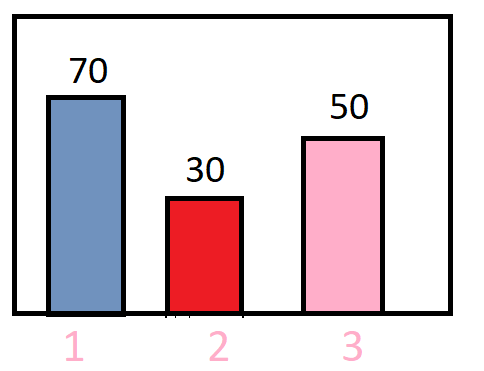
In the above distribution, random variable takes 3 values {1,2,3} with frequency {70,30,50} respectively. Our objective is to design a clustering model on the top of it.

Some of the key features of the data includes that it -
• Is discrete in nature
• Can be considered as a mixture of 2 probabilistic distribution functions

Since the objective is to find the parameters of the defined PDFs, let us first define our probability density functions as follows:

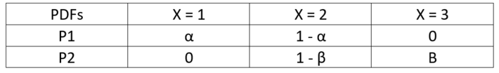
The above expression states that for PDF p1: random variable takes values {1,2,3} with probability { α , 1- α ,0 } respectively and similarly for PDF p2 : random variable takes values {1,2,3} with probability {0, 1 - β , β} respectively.

So now to be more precise we want to compute the exact values of α and β.

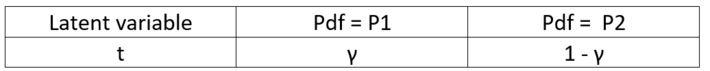
Let’s now introduce Latent Variable in the given scenario. As we need to apply the EM algorithm, we need a latent Variable.

Latent variable comes into the picture when we are unable to explain the behavior of the observed variable. In our case of clustering, we consider a latent variable t which defines which observed data point comes from which cluster or pdf function. In other words, how probable is a distribution.

Let us define the distribution of our latent variable t; we need to compute the values of γ, α and β.

Prior Setting

Let us first consider a prior value for all our variables
γ = α = β = 0.5
now the above equation states that:
P (X = 1 | t = P1) = 0.5
P (X = 2 | t = P1) = 0.5
P (X = 3 | t = P1) = 0
P (X = 1 | t = P2) = 0
P (X = 1 | t = P2) = 0.5
P (X = 1 | t = P2) = 0.5
P (t = P1) = 0.5
P (t = P2) = 0.5

E-Step

To solve the E step, we need to focus on the equation shown below:
q(t=c) = P(t=c | Xi , θ)
for i ranging for all the given data points.

Here q is the distribution from the lower bound after we use the Jensen’s inequality (refer post 5).

Let us compute the q(t=c) for all the given data points in our problem.
P(t=c | Xi ) = P(Xi | t = c)*P(t=c) / summation on c(P(Xi | t = c)*P(t=c))
P(t=1 | X =1 ) = (α * γ) / (α * γ + 0) = 1
P(t=1 | X =2 ) = ((1 – α) * γ) / ((1-α) * γ + (1- β)*(1- γ)) = 0.5
P(t=1 | X =3 ) = (0 * γ) / (0 * γ + (β)*(1- γ)) = 0
P(t=2 | X =1 ) = (0 * (1-γ)) / (0 * (1-γ)) + (α * γ)) = 0
P(t=2 | X =2 ) = (1- β)*(1- γ) / ((1- β)*(1- γ) + (1-α) * γ) = 0.5
P(t=2 | X =3 ) = (β)*(1- γ) / (β)*(1- γ) + 0 = 1

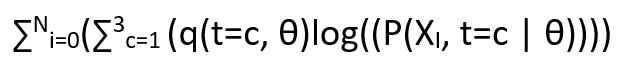
M Step

In the M step, we need to differentiate the below equation w.r.t γ ,α ,β and use the previously calculated values in E Step as constants. So the equation is :

We can ignore θ in the above representation for this problem as it is simple and disrete in nature with direct probabilities for 3 values.
So, now the new representation is as :
Likelihood lower bound differential part


To remember the above expression is simple:
Summation on datapoint(summation on q the values we computed in E step(log of joint distribution over Xi and t))
So, let us expand our equation, we will differentiate to compute our parameters


Solving the above equation by differentiating the equation 3 times, each time w.r.t 1 parameter and keeping the other 2 as constant we end up to the following result:
γ = (85/150), α = (70/85) , β = (50/65)
Now, again put the above computed parameter values in the E step for computation of the posterior and then perform M step again (in most of the cases the values do not change for a problem)
We do the above iterations until our parameter values stop updating.
And this is how we perform our EM algorithm.
Once we know the values of our parameters, we get to know our probability density function of P1 and P2. For any new value taken by our random variable X, we can specifically say from which cluster of pdf function it belongs and with what probability.

This point of view article originally published on datasciencecentral.com. Data Science Central is the industry's online resource for data practitioners. From Statistics to Analytics to Machine Learning to AI, Data Science Central provides a community experience that includes a rich editorial platform, social interaction, forum-based support, plus the latest information on technology, tools, trends, and careers.

Click here for the article